CS188 Chapter 15 Probabilistic Reasoning over Time

Notes CS188

---

Mark Chen | 15 Aug 2021

报告错误

如果你发现该网页中存在错误/显示异常，可以从以下两种方式向我们报告错误，我们会尽快修复：

1. 使用 CS Club 网站错误 为主题，附上错误截图或描述及网址后发送邮件到 286988023@qq.com
2. 在我们的网站代码仓库中创建一个 issue 并在 issue 中描述问题 点击链接前往Github仓库

belief state that represents which states of the world are currently possible. From belief state and a transition model, the agent can predict how the world might evolve in the next step.

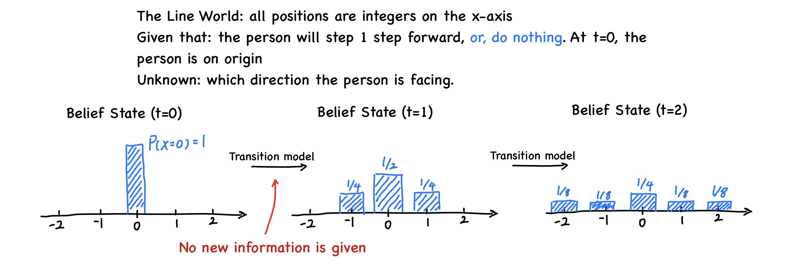
From information from the sensor model, agents can update the belief state.

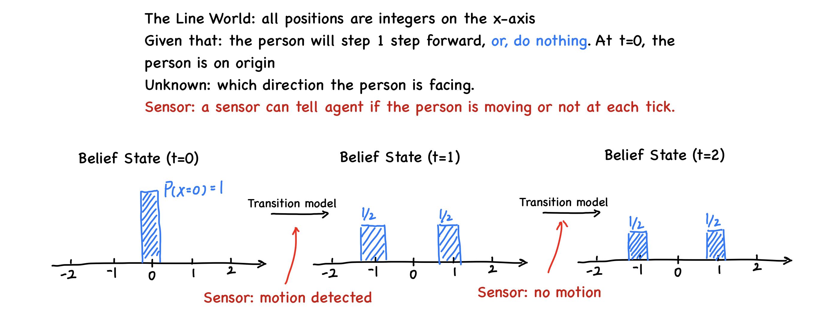
In previous section, belief state can only tell which state is possible, but can’t say which state is likely or unlikely. In this section, we can quantify the degree of belief in the belief state.

15.1 Time and Uncertainty

In previous section, we have talked about the Bayesian Network. Bayesian network can perform probabilistic reasoning in static world. The value of random variable at each moment is independent with its previous value.

However, in many scenario, the previous state DO influence the current state. To utilize such information, we use a model called Markov chain.

15.1.1 States and observations

We view the world as a series of snapshots (a.k.a. time slices and time is not continuous)

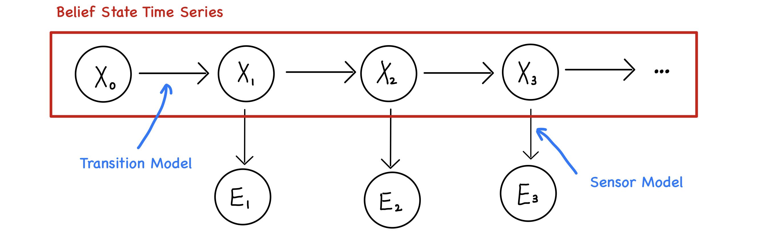
$\mathbf{X}_t$ denote the set of state variables at time $t$

$\mathbf{E}_t$ denote the set of observable evidence variables at time $t$

$\mathbf{E}_t = e_t$ where $e_t$​ is the observed value for evidence variable.

We will assume that the state sequence starts at $t=0$ and evidence starts arriving at $t=1$.

15.1.2 Transition and Sensor Models

Transition model specifies the probability distribution over the latest state variables given previous values, that is,

However, this leads to a problem: as $x\rightarrow \infty$, the size of set $\mathbf{X}_{0:t-1}$ has an unbounded size. To solve this problem, we introduce the Markov Assumption.

Process satisfying markov assumption is called Markov Process or Markov Chains.

Beyond first-order Markov process, there are second, third, …, n-th order Markov Process.

N-order Markov Process

Therefore, in a first-order Markov process, the transition model is the conditional distribution $\mathbf{P}(\mathbf{X_t}\mid \mathbf{X}_{t-1})$

Besides Markov Assumption, we also assume the world is stationary. At any given $t$, the transition model $\mathbf{P}(\mathbf{X_t}\mid \mathbf{X}_{t-1})$ is the same.

During the process, we can learn the status of world through sensor. The sensors read from world status and give us number. Therefore, it’s safe to assume that

$\mathbf{P}(\mathbf{E}_t \mid \mathbf{X}_t)$ is the Sensor Model, sometimes also called Observation Model.

15.1.3 Stationary State of Markov Model

In most cases, there exists a stationary state in the Markov Model, that is, there exists some distribution of probability of state $\mathbf{X}_ t$ such that $\mathbf{P}(\mathbf{X}_ t) = \mathbf{P}(\mathbf{X}_ {t+1})$

The state of Markov Model, in most cases, will converge to a stationary case.

15.1.4* Improve Markov Model?

Generally, there are two methods to increase the precision of Markov Model:

• Increase the order of Markov Process Model
• Increase the set of state variables.

By increasing the order of model, we can use information from multiple ticks to calculate the probability distribution on time $t$.

Increasing the order of model can always be reformulated as an increase in the set of state variables.

15.2 Inference in Temporal Models

There are four basic inference tasks that must be solved in generic temporal model:

• Filtering - computing the Belief State - the posterior distribution over the most recent state - given all evidence to date. $$\mathbf{P}(\mathbf{X_t}\mid e_{1:t})$$​

  With filtering, agent can keep track on current state and make rational decisions.

• Prediction - computing the posterior distribution over the future state, given all evidence to date.

  \[\mathbf{P}(\mathbf{X_{t+k}}\mid e_{1:t})\]

  Prediction is useful for evaluating possible courses of action based on their expected outcomes.

• Smoothing - computing the posterior distribution over a past state, given all evidence up to the present.

  \[\mathbf{P}(\mathbf{X}_k\mid e_{1:t}) , \text{where }1 \leq k\leq t\]

  Smoothing provides a better estimate of the state than was available at the time, because it incorporates more evidence.

• Most likely explanation - Given a sequence of observations, we might wish to find the sequence of states that is most likely to have generated those observations.

  \[\text{argmax}_{\mathbf{x}_{1:t}}P(\mathbf{x_{1:t}\mid e_{1:t}})\]

15.2.1 Filtering and Prediction

Filtering

Filtering algorithm should compute the probability distribution $\mathbf{P}(\mathbf{X}_ {t+1})$ from $\mathbf{P}(\mathbf{X}_ t\mid e _ {1:t})$ given new evidence $\mathbf{P}(e_ {t+1})$.

For function $f$, this process is called recursive estimation.

Below, we will reformulate the filtering function and find ways to describe filtering using sensor model, transition model etc.

1.Split the evidence $e_ {1:t+1}$ to $e_ {1:t}, e_ {t+1}$

2.Apply Bayes formula

Reference - Bayes Formula \(\mathbf{P}(\mathbf{X}_ {t+1}\mid e_ {1:t}, e_ {t+1}) = \frac {\mathbf{P}(e_ {1+t} \mid \mathbf{X}_ {t+1}, e_ {1:t})\mathbf{P}(\mathbf{X}_ {t+1} \mid e_ {1:t})} {\mathbf{P}(e_ {1+t}\mid e_ {1:t})}\)

Due to the sensor assumption in hidden markov model, $\mathbf{e_ {1+t}}$ is independent with $\mathbf{e_ {1:t}}$.

\[\mathbf{P}(\mathbf{X}_ {t+1}\mid e_ {1:t}, e_ {t+1}) = \frac {\mathbf{P}(e_ {1+t} \mid \mathbf{X}_ {t+1}, e_ {1:t})\mathbf{P}(\mathbf{X}_ {t+1} \mid e_ {1:t})} {\mathbf{P}(e_ {1+t})}\]

In this case, we change $\mathbf{P}(e_ {1+t})$ to normalization constant - $\alpha$.

3.Apply Sensor assumption in Hidden Markov Model

4.Expand the last term

In a short, we can filter on $\mathbf{X}_ {t+1}$ using this formula

$\mathbf{P}(\mathbf{X}_ {0}\mid e_ {1:0})$ is the probability distribution of state variable when NO CLUE is provided. Therefore, this value is a prior knowledge.

Prediction

By applying transition model repeatly, we can predict state at $t+2$, $t+3$, …, etc.

Case Study: Rain & Umbrella

You are in a basement and you want to know whether it is raining outside. The only information you can get is whether people get in basement with umbrella on their hands.

Prior Knowledge

• State transition model

  \[\mathbf{P}(R_t \mid R_ {t - 1}) = \left[\begin{matrix} P(\neg r_ t \mid r_ {t - 1}) = 0.3 & P(r_ t \mid r_ {t - 1}) = 0.7 \\ P(\neg r_ t \mid \neg r_ {t - 1}) = 0.7 & P(r_ t \mid \neg r_ {t - 1}) = 0.3\\ \end{matrix}\right]\]

  If it rains at day $t$, the probability to rain on day $t+1$ is 0.7, if …

• Sensor Model

  \[\mathbf{P}(u \mid R) = \left[\begin{matrix}0.9 & 0.2\end{matrix}\right]\]

  The probability of having an umbrella if rainy is $0.9$. However, even when it is not rainy, the probability of seeing an umbrella is $0.2$.

• Initial State Distribution

  On day 0, you believes $P(Rain) = P(\neg Rain) = 0.5$, in other words, $\mathbf{P}(R_0) = \langle0.5, 0.5\rangle$

Prediction & Filtering

Without any new information, you can predict $\mathbf{P}(R_1)$ by applying transition model.

Seems useless, ugh? But, things becomes interesting at the moment you receive new message: you see an umbrella so $U_1 = t$

Now we can run the filtering process:

15.2.2 Smoothing

Smoothing is computing the past state possibility distribution given all evidence. In formal mathematical language, smoothing is evaluating:

To evaluate this expression, we could take following steps:

1.Split the evidence variable set

2.Apply Bayes Rule, take $e_ {1:k}$​ as evidence variable set (Reference - Bayes Formula)

3.Accroading to sensor assumption in HMM, we know $e_ {k+1:t}$ is independent with $e_ {1:k}$

For the “Filtering” part, we can call filtering function described above. Below will discuss the “Backward” part. Backward function will broadcast information from “future” to the state we want to apply smoothing on.

1.Conditioning on $\mathbf{X}_ {k + 1}$

2.Conditional Independence

3.Split Evidence variables set

4.

We can find that $\mathbf {P}(e_ {k+1:t} \mid X_k)$’s expression contains $\mathbf {P}(e_ {k+2:t} \mid X_ {k + 1})$. So the evaluation process is a recursive process.

But there is one problem - as the size of evidence set increase, it will take increasing time to perform a smoothing operation (as it requires recursivly called from $k$ to $t$).

To solve this problem, a strategy called “fixed-lag smoothing” is proposed. For any $k$ that is called to smoothing on $X_k$, the Backward function will only called recursively to $k+n$ where $n$ is a constant.

15.2.3 Finding the most likely sequence

Sometimes, when we get a series of evidence value from sensor, we want to know the most-likely sequence of hidden state that can lead to such series of evidence value. Using mathematical language, we can describe finding most-likely sequence as such expression:

There is a recursive relationship between each state in the most-likely sequence.

评论区