CS188 Chapter 13 Quantifying Uncertainty

Notes CS188

---

Mark Chen | 30 May 2021

报告错误

如果你发现该网页中存在错误/显示异常，可以从以下两种方式向我们报告错误，我们会尽快修复：

1. 使用 CS Club 网站错误 为主题，附上错误截图或描述及网址后发送邮件到 286988023@qq.com
2. 在我们的网站代码仓库中创建一个 issue 并在 issue 中描述问题 点击链接前往Github仓库

13.1 Acting Under Uncertainty

An intelligent agent in reality needs to handle the uncertainty due to partial observability and nondeterminism.

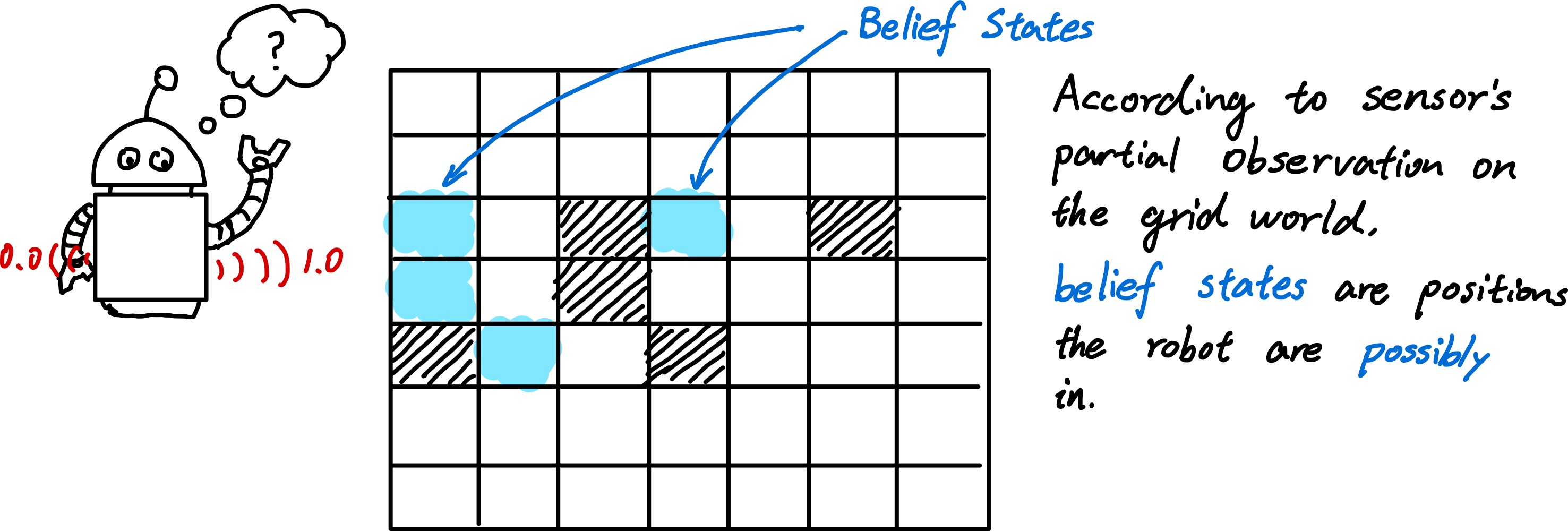
In previous chapters, agents handle uncertainty by keeping track of a belief state - a representation of the set of all possible states that it might be in.

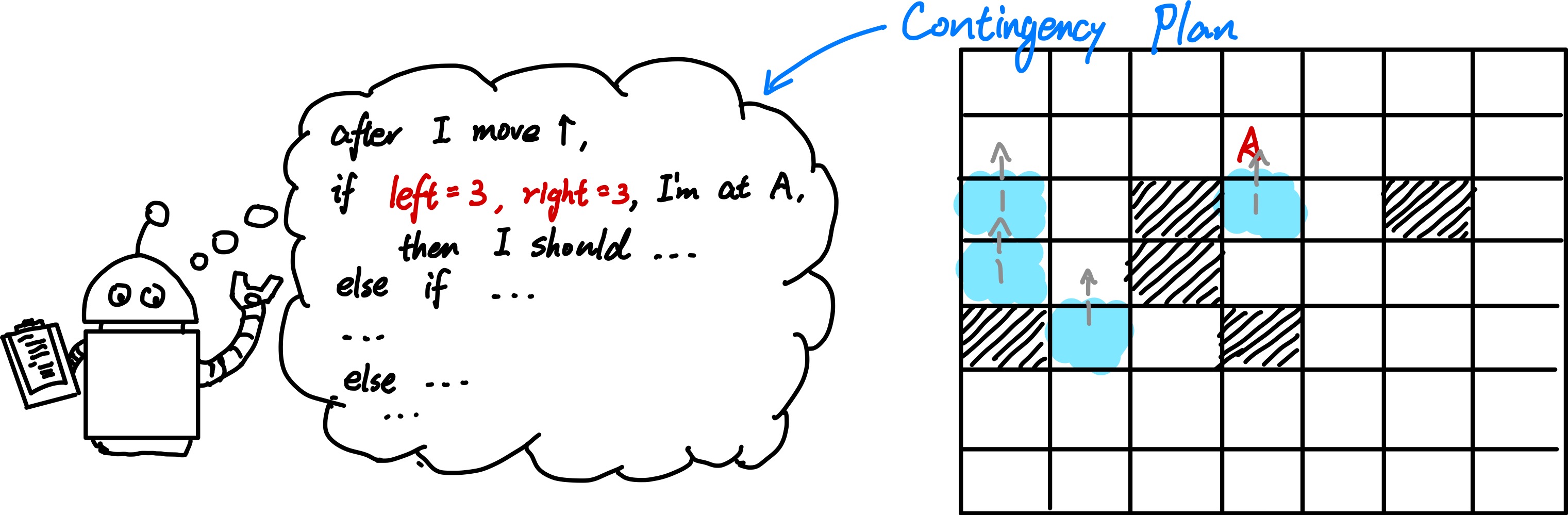
Based on the belief states, a contingency plan that handles every possible eventuality that its sensors may report during execution will be generated.

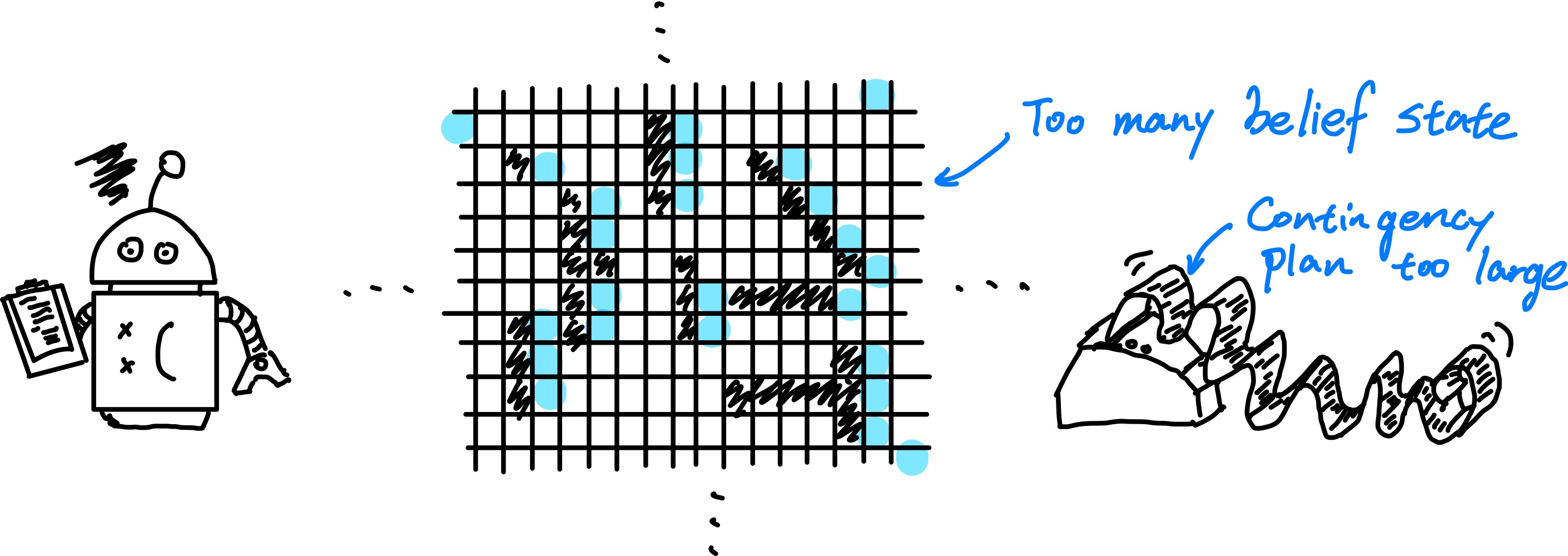
However, such method has significant draw back

• When interpreting partial sensor information, a logical agent must consider every logically possible explanation for the observations - this lead to impossibly large and complex belief state representations.
• A correct contingency plan handle every eventuality can grow arbitrarily large and must consider arbitrarily unlikely contingency.
• Sometimes, there does not exist a plan that is guaranteed to achieve the goal. However, agent should be able to compare the plans even if they are not guaranteed.

If we are using the belief state + contingency plan technique to solve real-world problem, the intelligent agent will hardly generate a valid solution. Suppose we want our agent plan the schedule to airport, the agent may think - “we should leave at 9 a.m. , as long as the weather is good”. Then, as the requirement of contingency plan is to handle all possible situation, it will begin to think - “what if the weather is bad”, “what if the bridge falls down due to storm”, “what if …” and finally reach a solution - “you should leave 2 months earlier to the airport to get there on time”.

So what’s the problem with this method? By definition, we should leave 2 months earlier to make sure we can arrive at the airport on time in any situation, but the question is - do we really need such certainty? Do we need to get to airport on time even if there is an earthquake? This leads to the concept of rational decision.

13.1.1 Summarizing uncertainty

Suppose an intelligent agent aims to get high GPA is deployed. The agent wants to list all the actions that will lead to low GPA:

It is clear that it is an almost unlimited list of possible problems that can cause Low GPA. Some people may try to reverse this logical relationship:

Which, unfortunately is also false, as not all low test score will lead to low GPA. So there does not exist a clear and definite logical relationship between $LowTestScore$ and $LowGPA$ anyway. In this situation, we need to describe the relationship between them using degree of belief, and solve problems using probability theory.

Probability provides a way of summarizing the uncertainty that comes from our laziness¹ and ignorance²

Probability statements are made with respect to a knowledge state, not with respect to the real world. When we say a student has a probability of $0.8$ to get low GPA, we are inference based on our knowledge state, not on the real world (as the student must either has high GPA or low GPA).

13.1.2 Uncertainty and Rational Decisions

Consider the airport schedule problem we mentioned above again. What should the agent choose as the final result? The one that leave 2 months ago and 100% make sure you arrive on time, or the one that leave 3 hours before the plane take off?

To make such choices, an agent must first have preferences between the different possible outcomes of the various plans. We use the utility theory to represent and reason with preferences.

Utility Theory: Every state has a degree of usefulness, or utility, to an agent and that the agent will prefer states with higher utility

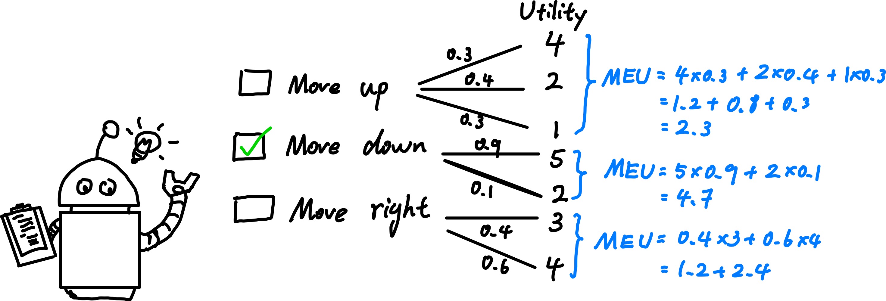
MEU is the statistical mean (expectation) of utility under best situation.

13.2 Probability Notation

13.2.1 What Probabilities are about

Probabilistic assertions talk about how probable the situation will occur. The set of all possible worlds is called the sample space ($\Omega$). The possible worlds are both exclusive and exhaustive - at any moment, there exist and only exist one world ($\omega$) as the actual world. \(0\leq P(\omega) \leq 1 \text{ for every } \omega \text{ and }\sum_{\omega\in\Omega}{P(\omega)} =1\)

Usually, we won’t use probabilistic assertions and queries on one particular possible worlds, but a set of them. For instance, we want to know the possibility of rolling two dices and their score sum up to 11. In Artificial Intelligence, such set is called a proposition ($\phi$).

Probabilities like $P(X=0)$ is called unconditional or prior probabilities (先验概率). It refer to degrees of belief in propositions in the absence of any other information. In most of the situations, we do have some known information before probabilistic query. Such information is called evidence, and the probabilities of event given the evidence is called conditional or posterior probabilities (后验概率).

When an agent make decision, all the evidence it observed will be the evidence and used to calculate the posterior probabilities.

When we say $P(X=0\mid 0\leq X \leq 5)$ , it means that - “the probability of $X=0$ given $0\leq X\leq 5$ and no further information”.

13.2.2 The Language of propositions in Probability Assertions

Variables in probability theory are called random variables. Every random variables has a domain - the set of all valid value a random variable can be assigned to.

When we want to talk about the probabilities of all the possible values of a random variable, we can use the $\mathbf{P}$ notation.

Example:

\[P(Weather=sunny) = 0.6\\ P(Weather = rain) = 0.1\\ P(Weather = cloudy) = 0.29\\ P(Weather = snow) = 0.01\]

In this case, we can simplify it to this form:

\[\mathbf{P}(Weather) = \langle 0.6, 0.1, 0.29, 0.01 \rangle\]

The $\mathbf{P}$ statement defines the probability distribution for random variable.

$\mathbf{P}(X\mid Y)$ can represent the conditional distribution of $X$ and $Y$ - that is, the value of $P(X=i \mid Y=j)$ for all possible $i, j$ pairs.

$\mathbf{P}(X, Y)$ is called the joint distribution - which represent the possibility of $P(X=i \wedge Y=j)$ for all valid value pairs $i, j$.

A possible world is defined to be an assignment of values to all of the random variables under consideration.

The full joint probability distribution is the joint probability distribution with all random variable in consideration.

13.3 Inference using Full Joint Distribution

In this section, we describe a simple method for probabilistic inference - the computation of posterior probabilities for query propositions given observed evidence.

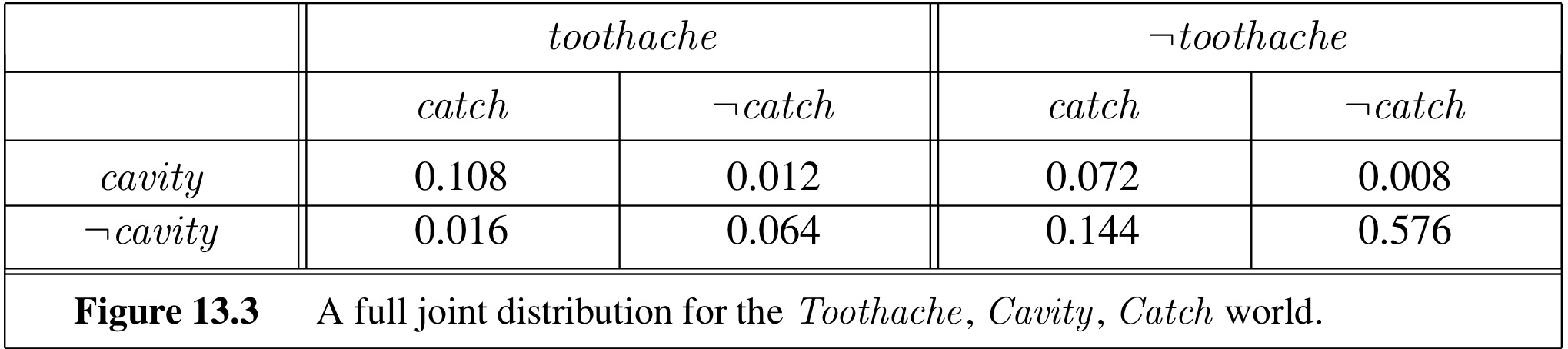
Suppose we have a domain only has three Boolean variables $Toothache$, $Cavity$ and $Catch$. The table above shows $\mathbf{P}(Cavity, Catch, Toothache)$.

The first type of probabilistic inference is to calculate the marginal probability of random variable, i.e., the unconditional probability distribution of random variable. In this Example, we can query for $\mathbf{P}(Cavity)$.

This process is called marginalization - sum up the probabilities for each possible value of the other variables, thereby taking them out of the equation.

In the example above, we can rewrite the calculation into the “standard” form:

A variant of this rule involves conditional probabilities instead of joint probabilities - using the Product rule.

In most cases, we are interested in computing conditional probabilities of some variables given evidence about others.

Using Equation \(P(A\mid B) = \frac{P(A \wedge B)}{P(B)}\), we can calculate the conditional probability from unconditional probability and joint probability.

In the example above, we can evaluate the probability of $cavity$ given $toothache$.

During the calculation, we notice that both $P(cavity\mid toothache)$ and $P(\neg cavity \mid toothache)$ is multiplied by a factor of $\frac{1}{P(toothache)}$. We call the value of $\frac{1}{P(toothache)}$ the normalization constant, denote as $\alpha$.

Combining the Marginalization and Normalization, we can get a general equation to evaluate conditional probability from joint distribution.

Given the full joint distribution table, the equation above is able to answer any probabilistic queries for random variables. However, it does not scale well. If there are $n$ random boolean variables to consider, the size of joint distribution table will be $O(2^n)$ and takes $O(2^n)$ time to process the table.

To solve this problem, we will use the tool of independence to simplify the relationship between random variables.

13.4 Independence

To begin with, let’s see back this case again and adding a fourth random variable $Weather = \lbrace sunny, cloudy \rbrace$.

How are $P(toothache, catch, cavity, cloudy)$ related with $P(toothache, catch, cavity)$ related? According to the Conditioning Rule, we can know that

To write in General form with $\mathbf{P}$ notation

Since we don’t expect the evidence on $Weather$ affect the probability distribution of $Toothache, Catch ,Cavity$, it is clear that

Therefore, we can say

This situation is called independence. Formally speaking, $A$ and $B$ are independent if and only if

Except the equation above, there are also other ways to represent the independence between random variable $A$ and $B$:

By separating the independent random variables from all considered random variables, we can factored the full joint distribution into several independent joint distribution tables.

Example: Suppose we have $n$ coins that are denoted as $C_1$, $C_2$, $\cdots$, $C_n$. If we want to build up a full-joint distribution table, the table will contain $2^n$ entries.

\[\mathbf{P}(C_1, C_2, \cdots, C_n) \overrightarrow{\text{ factor }}\lbrace \mathbf{P}(C_1), \mathbf{P}(C_2), \cdots, \mathbf{P}(C_n)\rbrace\]

However, since every coin’s state is independent with other coins, we can factor the full-joint distribution table into $n$ joint-distribution table, each represent the state of a single coin and independent with each other.

13.5 Bayes’ Rule and Its Use

In previous section, we have introduced the product rule - $P(a\wedge b) = P(a \mid b)P(b)$ and its second form - $P(a\wedge b) = P(b\mid a)P(a)$.

Combining these two forms together and divide both sides by $P(a)$, we get

It also has a more general rule with some background condition $e$.

13.5.1 Applying Bayes’ Rule: The simple case

In real-world application, we usually see evidence as the $effect$ of some unknown $cause$ and we would like to determine the cause from effect. In this situation, the Bayes’ rule becomes

Evaluation of $P(effect\mid cause)$ quantifies the relationship in causal direction (因果关系)

Evaluation of $P(cause \mid effect)$ quantify the relationship in diagnostic direction

Example

Suppose we know that $P(cough) = 0.1$ and $P(covid) = 0.001$. By checking each Covid-19 patient separately, we learn that $P(cough \mid covid) = 0.6$. Now we want to evaluate $P(covid \mid cough)$.

\[P(covid \mid cough) = \frac{P(cough \mid covid) P(covid)}{P(cough)} = \frac{0.6\times 0.001}{0.1} = 0.006\]

However, sometimes it is hard to get the prior probability of evidence (in this case, $P(cough)$).

In this case, we can still find out $P(covid\mid cough)$ by bypassing $P(cough)$ using normalization.

\[\mathbf{P}(Covid \mid cough) = \alpha \langle P(cough \mid covid)P(covid), P(cough, \neg covid)P(\neg covid)\rangle\]

Where $\alpha$ is the normalization constant that makes $\mathbf{P}(Covid \mid cough)$ sum up to $1$.

13.5.2 Using Bayes’ rule: Combining Evidence

We introduced the independence between random variables before, but here, we will introduce a new kind of independence - conditional independence.

$X$ and $Y$ are conditional independence if and only if

Suppose we have one $cause$ and several $effects$, we can calculate the joint distribution of

Such a probability distribution is called Naïve Bayes - it is “naive” since it is often used (as simplification) in cases where the effect variables are not actually conditionally independent with each other.

Notes

评论区