
报告错误
如果你发现该网页中存在错误/显示异常,可以从以下两种方式向我们报告错误,我们会尽快修复:
- 使用 CS Club 网站错误 为主题,附上错误截图或描述及网址后发送邮件到 286988023@qq.com
- 在我们的网站代码仓库中创建一个 issue 并在 issue 中描述问题 点击链接前往Github仓库

14.1 Representing Knowledge in an Uncertain Domain
This section will introduce a data structure called Bayesian network to represent the dependencies between variables. Bayesian network can represent any full-joint probability distribution and in many cases can do so very concisely.
A Bayesian network is a directed acyclic graph (DAC) where each node is annotated with quantitative probability information.
- Each node corresponds to a random variable, which may be discrete or continuous.
- A set of directed links or arrows connects pairs of nodes. If there is an arrow from node $X$ to $Y$, $X$ is said to be a parent of $Y$.
- Each node $X_i$ has a conditional probability distribution $\mathbf{P}(X_i\mid Parents(X_i))$ that quantifies the effect of the parents on the node.
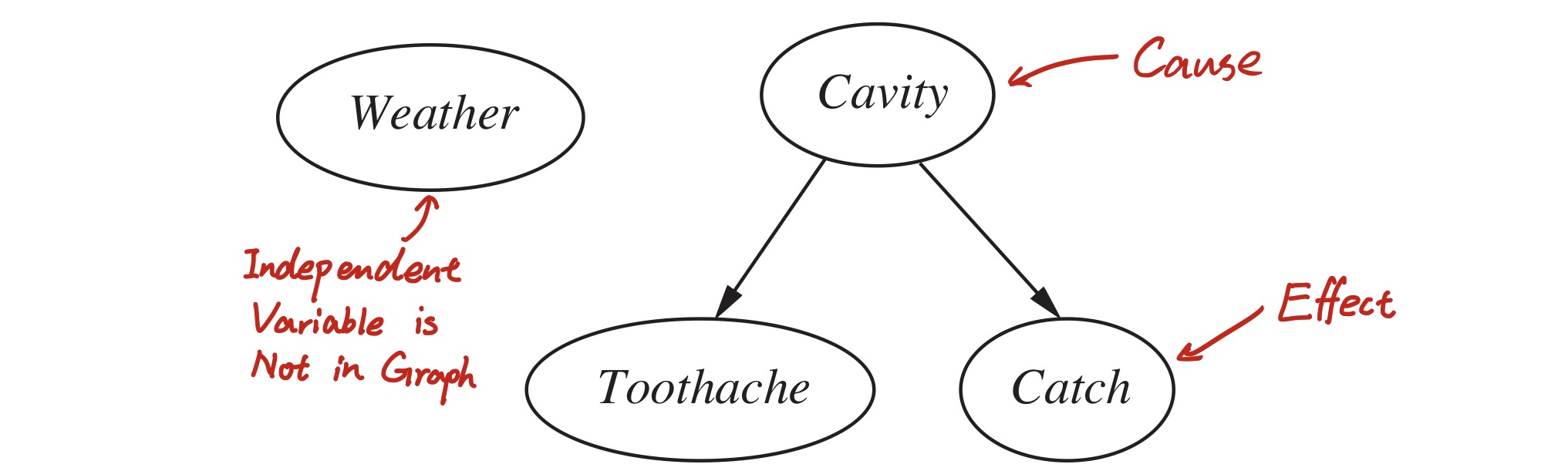
In each node of the Bayesian network, a conditional probability table (CPT) is stored. For instance, the node “$Toothache$” stores $\mathbf{P}(Toothache \mid Cavity)$.
In general, a table for a Boolean variable with $k$ Boolean parents contains $2^k$ independently specifiable probabilities.
14.2 The Semantics of Bayesian Networks
14.2.1 Representing the full joint distribution
The full joint distribution of variables $X_1$ to $X_n$ can be represented in this way:
\[P(x_1, \cdots, x_n) = \prod_{i=1}^{n}{P(x_i \mid parents(X_i))}\]Where $parents(X_i)$ is the parent nodes of variable $X_i$.This equation defines what a given Bayesian network means.
How to construct Bayesian Networks
Except the equation above, there is another way to calculate $P(x_1, \cdots, x_n)$. Using product rule, we can also represent it in this way:
\[P(x_1, \cdots, x_n) = P(x_n \mid x_{n-1}, x_{n-2}, \cdots, x_1)P(x_{n-1}, x_{n-2}, \cdots, x_1)\]Applying product rule recursively on the equation above, we can represent $P(x_1, \cdots, x_n)$ in a long product:
\[P(x_1, \cdots, x_n) = P(x_n \mid x_{n-1}, x_{n-2}, \cdots, x_1)P(x_{n-1} \mid x_{n-2}, \cdots, x_1)\cdots P(x_2 \mid x_1)P(x_1) \\= \prod_{i=1}^{n}{P(x_i \mid x_{i-1} \cdots x_1)}\]Therefore, we can learn that[图片]
\[P(X_i\mid X_{i-1}. \cdots. X_i) = P(X_i \mid parents(X_i))\]This equation indicates that …
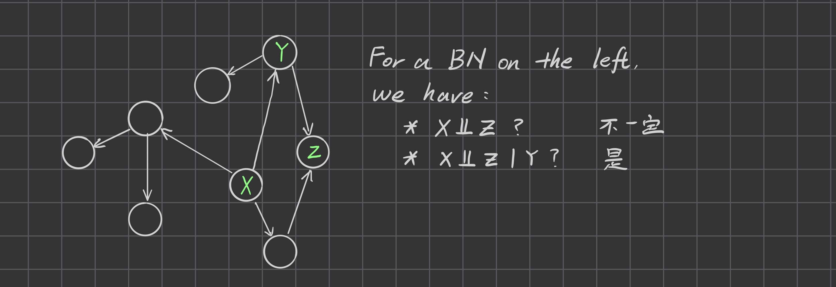
\(P(X\mid Parents(X))\;\bot\; P(Ancestor(X) \mid Parents(X))\)
- Nodes: First find a set of variables $X_1, \cdots, X_n$ that will be included into the Bayes Network. The network will be more compact if the variables are ordered such that cause precede effect
-
Links For $i = 1$ to $n$, do
- Choose from $X_1, \cdots, X_{i-1}$ a minimal set of parents for $X_i$, such that Equation $P(X_i\mid X_{i-1}. \cdots. X_i) = P(X_i \mid parents(X_i))$ is satisfied.
- For each parent insert a link from parent to $X_{i}$
- Write down the conditional probability table, $\mathbf{P}(X_i \mid Parents(X_i))$
14.4 Exact Inference in Bayesian Networks
The basic task for probabilistic inference system is to compute the posterior probability distribution for a set of query variables, given some observed event (the assignment of values to a set of evidence variables).
\[\text{All Variables} = \text{Query Variables }\cup\text{ Evidence Variables }\cup\text{ Hidden Variables}\]A typical query asks for the posterior probability distribution $\mathbf{P}(X\mid \mathbf{e})$
14.4.1 Inference by Enumeration
A query $\mathbf{P}(X \mid \mathbf{e})$ can be answered using the equation below:
\[\mathbf{P}(X \mid \mathbf{e}) = \alpha \mathbf{P}(X, \mathbf{e}) = \alpha \sum_y{\mathbf{P}(X,\mathbf{e}, \mathbf{y})}\]a query can be answered using a Bayesian Network by computing sums of products of conditional probablities from the network.
Example
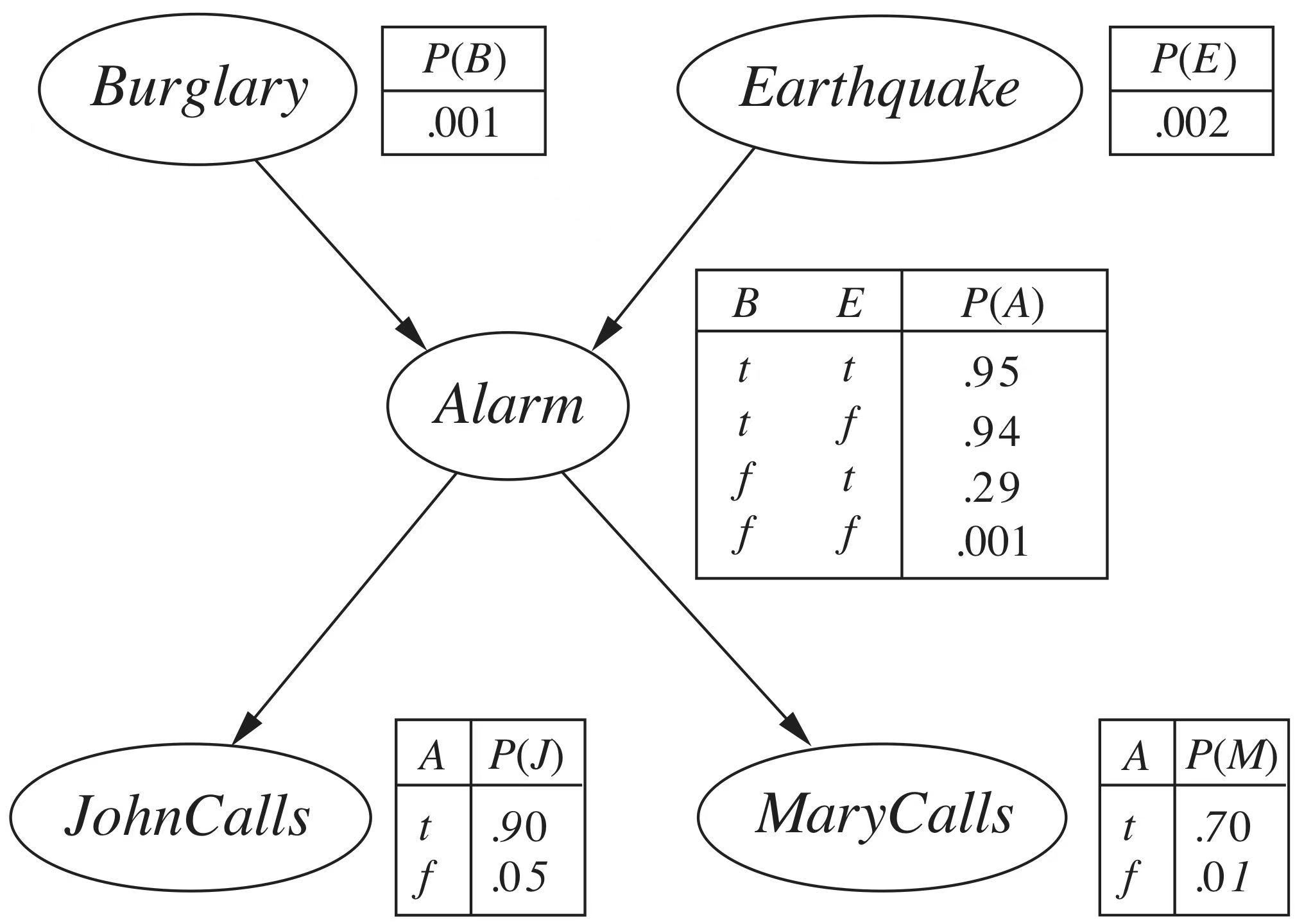
Suppose we have such a Bayesian Network
We use $B$ to represent the variable $Burglary$, $m$ and $j$ represent the known value of $JohnCalls$ and $MaryCalls$ (True or False). Now we want to calculate $\mathbf{P}(B\mid m, j)$
\[\begin{aligned} \mathbf{P}(B\mid m, j) &= \left\langle \frac{P(b, j, m)}{P(j, m)}, \frac{P(\neg b, j, m)}{P(j, m)} \right\rangle\\ &= \alpha \left\langle \underbrace{P(b, j, m)}_{\text{Expand}}, P(\neg b, j, m)\right\rangle \end{aligned}\]Using Chain Rule, we can expand $P(b, j, m, E, A)$
\[\begin{aligned} P(b, j, m) &= \sum_E{\sum_A{P(b, j, m, E, A)}}\\ &= \sum_E{\sum_A{P(m \mid j, A, E, b)P(j \mid A, E, b)P(A \mid E, b)P(E\mid b)P(b)}} \end{aligned}\]Note: For simplicity
$x\bot y$ is the shorten for $P(x)\bot P(y)$
$x\bot y \mid a$ is the shorten for $P(x\mid a) \bot P(y\mid a)$
$x\bot y, z \mid a$ is the shorten for $P(x\mid a)\bot P(y\mid a)$ and $P(x\mid a)\bot P(z\mid a)$
According to the structure of Bayesian Network, we can know that $m \bot j$, $m \bot b, E \mid A$, $j \bot b, E \mid A$ and $b\mid E$. Therefore, we can simplify the formula above
\[\begin{aligned} P(b, j, m) &= \sum_E{\sum_A{P(m \mid j, A, E, b)P(j \mid A, E, b)P(A \mid E, b)P(E\mid b)P(b)}}\\ &= \sum_E{\sum_A{P(m\mid A)P(j \mid A)P(A\mid E, b)P(E)P(b)}} \end{aligned}\]To simplify this formula, we can “extract the common factor” out from nested sum$\sum$.
\[\begin{aligned} &P(b, j, m)\\ = &P(b)\sum_E\left({P(E)\sum_A\left({P(m \mid A)P(j\mid A)P(A\mid E, b)}\right)}\right)\\ = &P(b)\sum_E\left({P(E)\sum_A\left({\underbrace{P(m\mid Parents(m))P(j\mid Parents(j))P(A\mid Parents(A))}_{\text{Find these value in Bayesian Network}}}\right)}\right) \end{aligned}\]
The worst time complexity of query with enumeration is $O(n2^n)$
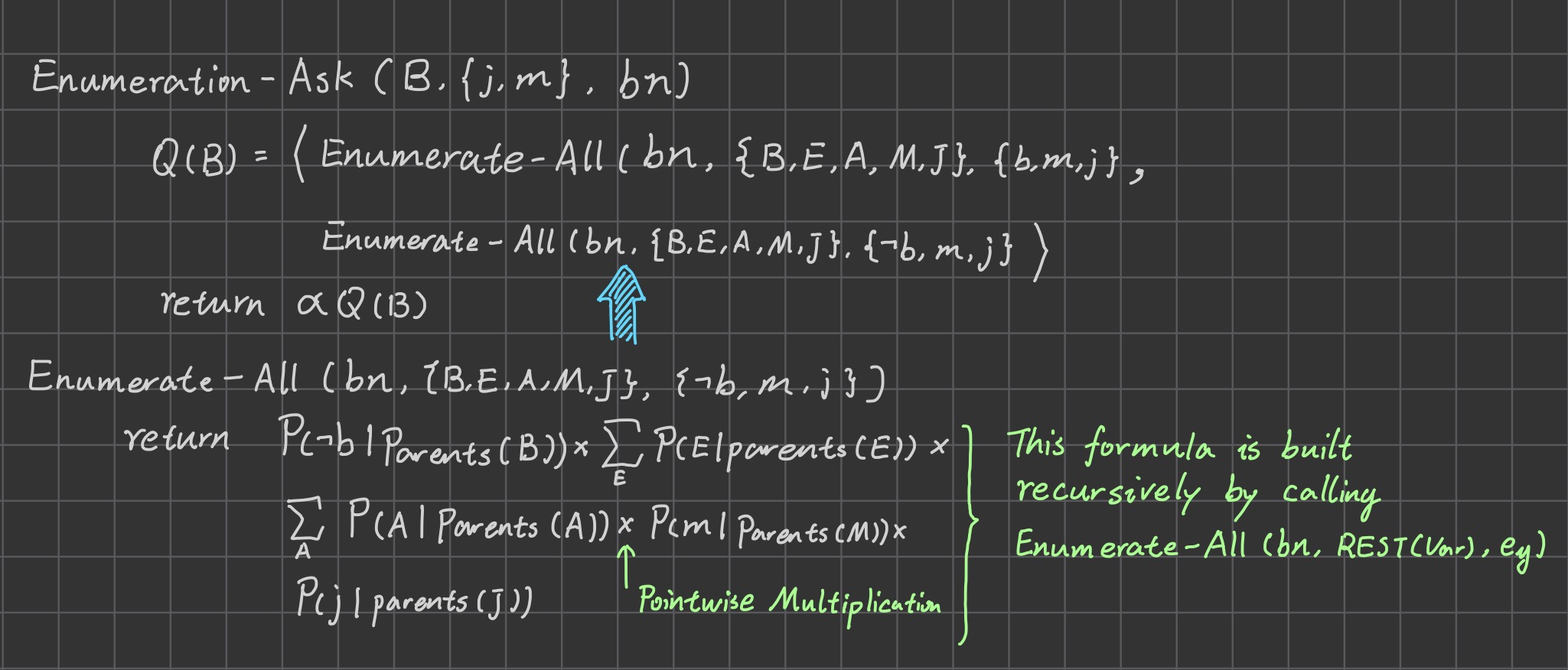
To formally describe the process of Inference by Enumeration, we can use two functions - $\text{ENUMERATION-ASK}$ and $\text{ENUMERATE-ALL}$.
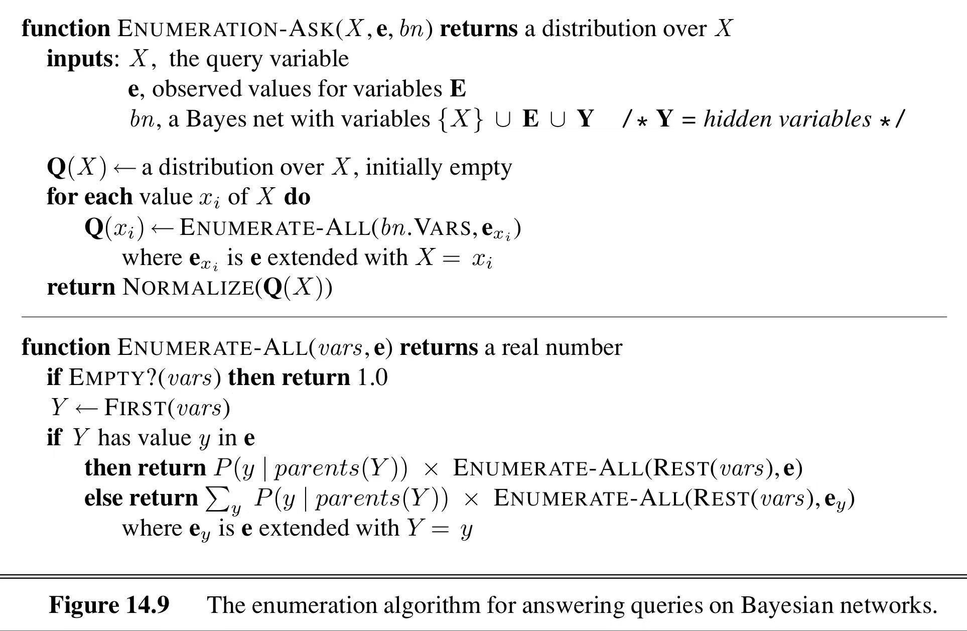
The $\times$ here represents the pointwise product between vectors instead of scalar product.
Here’s how to use $\text{ENUMERATION-ASK}$ and $\text{ENUMERATE-ALL}$ to evaluate $\text{ENUMERATION-ASK}(B, \lbrace j,m\rbrace, bn)$.
14.5 Approximate Inference in Bayesian Networks
This section describes randomized sampling algorithms, also called Monte Carlo algorithms, that provide approximate answers whose accuracy depends on the number of samples generated.
14.5.1 Direct Sampling Methods
Prior Sample
Step 1. Use topological sort to sort all variables in the Bayesian Network.
Step 2. Assign a value to the first variable (the node with no Parents) randomly with probability distribution $\mathbf{P}(X_1)$.
Step 3. Assign a value to next variable with probability distribution $\mathbf{P}(X_2 \mid Parents(X_2))$
Step 4. Repeat Step 3 until all variables in Bayesian Network has an assignment
After step 4, we successfully construct a sample from Bayesian network. By repeating the sampling for many times, we can approximate the Probability distribution $\mathbf{P}(X\mid e)$.
Suppose $S_{PS}(x_1, \cdots, x_n)$ represents the probability of getting sample where $X_1 = x_1, \cdots, X_n=x_n$.
\[S_{PS}(x_1\cdots x_n) = \prod_{i=1}^n{P(x_i\mid Parents(X_i))}\]Suppose we have take $N$ direct samples and among them, there are $N_{PS}(x_1\cdots x_n)$ sample where $X_1=x_1\cdots X_n=x_n$. The ration between $N$ and $N_{SP}$ will converge as $N$ approach $\infty$.
\[\lim_{N\rightarrow\infty}{\frac{N_{PS}(x_1\cdots x_n)}{N}} = S_{PS}(x_1, \cdots, x_n)=P(x_1, \cdots, x_n)\]The estimated probability becomes exact in the large-sample limit. Such an estimate is called consistent.
\[P(x_1, \cdots, x_m)\approx N_{PS}(x_1, \cdots, x_m)/N\]Rejection Sampling
Rejection sampling is a general method for producing samples from a hard-to-sample distribution given an easy-to-sample distribution. It can produce a consistent estimation of the true probability.
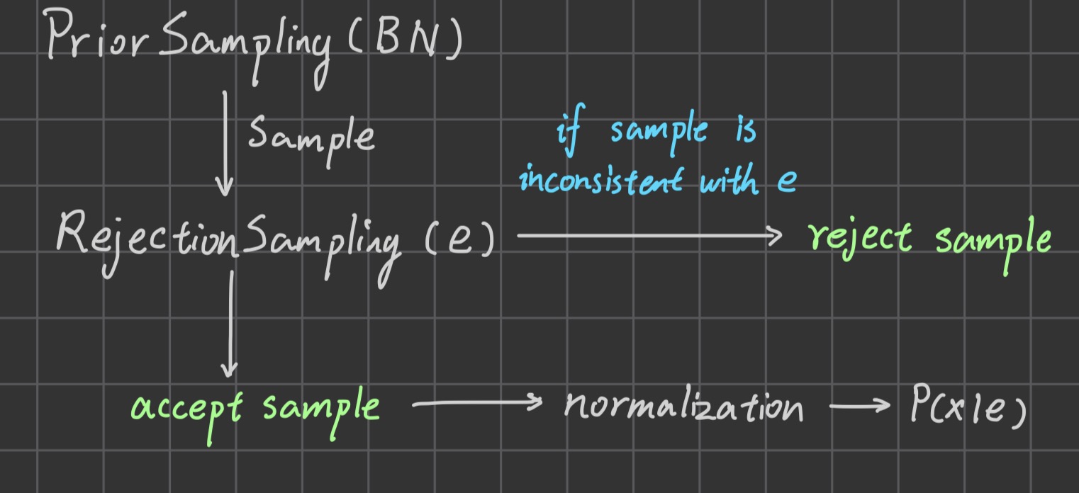
The biggest problem of rejection sampling is that it rejects too much samples! The number of samples being rejected increases exponentially as the number of evidence variable increases.
