
报告错误
如果你发现该网页中存在错误/显示异常,可以从以下两种方式向我们报告错误,我们会尽快修复:
- 使用 CS Club 网站错误 为主题,附上错误截图或描述及网址后发送邮件到 286988023@qq.com
- 在我们的网站代码仓库中创建一个 issue 并在 issue 中描述问题 点击链接前往Github仓库

开始之前……
先下载 Case Study Package,其中包括了 Jupyter Notebook 文件,MNIST 数据集,和 Python 文件
提取码:gwcs
Using Naive Bayes’ Network to Recognize MNIST Handwriting Figures
This dataset contains two files - mnist_test.csv and mnist_train.csv. They are in the data directory. You can also download them from this link
What is MNIST?
MNIST is a set of hand-writing images collected by NIST. Each image is cropped to $28px \times 28px$. There exist a single digit in each image.
The image is gray-scaled. Each pixel has a value in range $[0, 255]$. Where $0$ represents “white” and $255$ represents “black”.
Now, let’s take a look at MNIST first.
def load_csv(pathToCSV: str) -> list:
    """
    加载 csv 数据
    """
    data = []
    lines = open(pathToCSV, "r").read().strip().split("\n")
    data = [list(map(int, line.split(","))) for line in lines]
    return data

train_set = load_csv("./data/mnist_train.csv")      # 训练集,共 60,000 张(行)
test_set = load_csv("./data/mnist_test.csv")        # 测试集,共 10,000 张(行)

def display_image(pixels: list) -> None:
    """
    Display the image using ASCII char, also show the label on image
    """
    assert len(pixels) == 1 + 28 * 28, "Unable to display image other than size 28 * 28 and 1 label"
    gray_chars = " .:-=+*#%@"
    gray_scale = 9
    print("Label: {}".format(pixels[0]))
    for index, pixel in enumerate(pixels[1:]):
        if(index % 28) == 0: print()
        print(gray_chars[pixel * gray_scale // 255], end=" ")
    print("\n")
Code:
display_image(train_set[1])
Output:
Label: 0


                              . + % + .
                            . % % % % %
                          . % % % % % % :
                        : # % % % # : % % =
                      + % % % % % % - * % +
                    . % % % * = % % . : @ +
                  . % % % *   : =       % % .
                . + % % # :             % % +
                * % % :                 % % *
              : % % :                   % % *
              * % *                     @ % *
            : % % -                     % % +
            - % %                     = % *
            - % #                   = % # :
            - % +               . + % *
            - % #             = % % +
            - % % + . . - * # % # + .
            - % % % % # % % % * =
              # % % % % % % +
                = % % % = .
Simplification on image: Binarization
To further simplify the model (and reduce the memory requirement of naive bayes classifier), we can binarize the image.
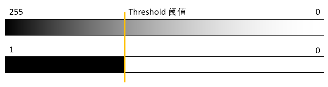
def binarize_image(pixels: list, threshold=120):
    """
    [Label, Pixel 1, Pixel 2, ..., Pixel 784]
    """
    binaryImg = [pixels[0]] # include the label
    binaryImg += [0 if pixel < threshold else 1 for pixel in pixels[1:]]    # binarize image based on threshold
    return binaryImg

def display_binary_image(pixels: list):
    display_image([pixels[0]] + [pixel * 255 for pixel in pixels[1:]])

binary_train_set = [binarize_image(img) for img in train_set]
binary_test_set = [binarize_image(img) for img in test_set]
Code:
display_binary_image(binarize_image(train_set[5]))
Output:
Label: 2


                                    @
                            @ @ @ @ @ @
                        @ @ @ @ @ @ @ @
                    @ @ @ @ @ @     @ @
                    @ @ @ @ @       @ @
                  @ @ @ @ @         @ @
                    @               @ @
                                  @ @ @
                            @ @ @ @ @ @
                        @ @ @ @ @ @ @
                    @ @ @ @ @ @ @ @ @
                  @ @ @       @ @ @ @ @
              @ @ @ @       @ @ @ @ @ @ @ @
            @ @ @         @ @ @         @ @ @ @ @
            @ @       @ @ @ @               @ @
          @ @ @ @ @ @ @ @ @
          @ @ @ @ @ @
              @ @
Bayes Network on Image Recognition?
To begin with, we assume that the binary values on pixel are conditionally independent under the condition of label.
\[\mathbf{P}(Pixel_1 \mid Label) \bot \mathbf{P}(Pixel_2 \mid Label) \bot ... \mathbf{P}(Pixel_{784} \mid Label)\]Since we know the input image, we know the value of each pixel, we can easily calculate $\mathbf{P}(pixel_1, pixel_2, \cdots ,pixel_{784} \mid Label)$ using this equation:
\[\mathbf{P}(pixel_1, pixel_2, \cdots, pixel_{784} \mid Label) = \prod_{i \in [1, 784]}{\mathbf{P}(pixel_i \mid Label)}\]For simplicity, use $X$ denotes for $\lbrace pixel_1, pixel_2, \cdots, pixel_{784} \rbrace$
\[\begin{aligned} \mathbf{P}(Label \mid X) &= \alpha \mathbf{P}(X \mid Label)\mathbf{P}(Label)\\ &= \alpha \langle P(X \mid label_0)P(label_0), P(X\mid label_1)P(label_1), \cdots, P(X\mid label_9)P(label_9)\rangle\\ &= \alpha \langle \prod{P(pixel_i \mid label_0)\cdot P(label 0), \cdots}\rangle \end{aligned}\]LabelCount = [0] * 10 # Counter for Label, used to calculate P(Label)
PixelCount = [[0] * 784 for _ in range(10)] # Counter for Pixel | Label, used to calculate P(pixel | label)
for img in binary_train_set:
LabelCount[img[0]] += 1
for index in range(1, len(img)): PixelCount[img[0]][index - 1] += img[index] # +1 if pixel is black, 0 otherwise
LabelDistribution = [LabelCountElem / len(train_set) for LabelCountElem in LabelCount]
PixelDistribution = [
[ pixel / LabelCount[i] for pixel in PixelCount[i]]
for i in range(10)]
Code:
print("Label Distribution:\n", LabelDistribution)
Output ($\mathbf{P}(Label)$):
Label Distribution:
 [0.09871666666666666, 0.11236666666666667, 0.0993, 0.10218333333333333, 0.09736666666666667, 0.09035, 0.09863333333333334, 0.10441666666666667, 0.09751666666666667, 0.09915]
With the statistical data collected from the Training set, we can now construct our Naive Bayes classifier.
def get_pixel_prob(index, value, label):
    global PixelDistribution
    try:
        black_probability = PixelDistribution[label][index]
    except:
        print(label, index)
    if value: return black_probability
    return 1 - black_probability

def predict_image(pixels):
    global PixelDistribution, LabelDistribution
    assert len(pixels) == 784, "only predict image without label at 0"
    pred_probability = [0] * 10
    for pred_label in range(10):
        posterior_probability_list = [get_pixel_prob(index, value, pred_label) for index, value in enumerate(pixels)]
        posterior_probability = 1
        for prob in posterior_probability_list: posterior_probability *= prob
        # posterior_probability = \prod{P(pixel_i | label_pred)}
        pred_probability[pred_label] = posterior_probability * LabelDistribution[pred_label]
    alpha = sum(pred_probability)
    return [prob / alpha for prob in pred_probability]
Classification on Test Set
Code:
selected_image_index = 3101
print("Predict Probability:\n", list(predict_image(binary_test_set[selected_image_index][1:])))
display_image(test_set[selected_image_index])
Output:
Predict Probability:
 [0.0, 0.0, 0.0, 1.3577222853703937e-55, 2.3620356632673247e-37, 1.0415370695140759e-36, 0.0, 0.9999999999999999, 6.262374232930145e-42, 1.1556946478312145e-16]
Label: 7


                  + + - . : + + * % % % *
                * % % % % % % % % % % % % =
                # @ % % % % % % % % % % % % .
              . % % % % % % % + - - * % % % .
                # @ % % % +         = % % #
                = % % % % :       . % % % =
                . % % % +         + % % %
                  : + = .       . % % % *
                                # % % #
                              * % % % =
                            * % % % =
                          - % % % *
                        : % % % *
                        # % % * .
                    . * % % %
                    # % % % *
                  - % @ % #
                  * % % % #
                  % % @ % *
                  . * % +
