
报告错误
如果你发现该网页中存在错误/显示异常,可以从以下两种方式向我们报告错误,我们会尽快修复:
- 使用 CS Club 网站错误 为主题,附上错误截图或描述及网址后发送邮件到 286988023@qq.com
- 在我们的网站代码仓库中创建一个 issue 并在 issue 中描述问题 点击链接前往Github仓库

5.1 Games
This chapter describes the Competitive Environments for agents, where their goals are conflict. Such problem is called the adversarial search problems - often known as games.
In the field of AI, the most common games are a special kind of game - the Deterministic, Turn-taking, Two-player, Zero-sum games of Perfect Information (such as chess).
Games are interesting since they are hard to solve using direct search - the branching factor of game is too large that it is impossible to search through all possible states. Also, games penalize inefficiency severely so the program should be as fast as possible.
Pruning (剪枝) allows us to ignore portions of search tree that make no difference to the final choice. Heuristic Evaluation Functions allow us to approximate the true utility of a state without doing a complete search.
Suppose there are two agents - “MAX” and “MIN”. In a game, “MAX” move first and they take turn to move until the game is over. The winner get points and loser get penalty.
5.1.1 Formally Defined Game
A game can be formally defined with these elements
| Element | Explanation |
|---|---|
| $S_0$ | The Initial State of game (the setup of game) |
| $Player(s)$ | Defines which player has a move in the current state $s$ |
| $Actions(s)$ | Returns a list of legal actions in a state $s$ |
| $Result(s, a)$ | The state transition model, which defines the result of an action $a$ |
| $Terminal-Test(s)$ | Returns true if the game is over, false otherwise |
| $Utility(s, p)$ | A utility function defines the numeric value for a game that ends in terminal state $s$ for player $p$ |
The Zero-sum game is defined as one where the total payoff to all players is the same for every instance of the game.
The initial state $S_0$, $Action$ function and $Result$ function define the game tree for the game - a tree where the nodes are game states and the edges are actions.
In a game tree, we record the utility value of the terminal state from the point of view of $MAX$ agent.
Though a game tree is well-defined and has finite amount of nodes in it, it is better thought to be a theoretical construct we can’t realize in physical world as it has too many nodes in it (the Go has $10^40$ nodes, tic-tac-toe has more than $3\times 10^5$ nodes). We usually use term search tree to represent a tree that is extracted from the full game tree, and contains enough nodes to allow a player to determine what action to make.
5.2 Optimal Decision in Games
In an adversarial search scene, the MAX agent must find a contingent strategy. An optimal strategy leads to outcomes at least as good as other strategy when one is playing an infallible opponent.
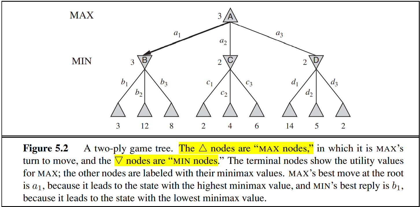
In the graph above, the maximum utility at node $A$ is 3, since the MAX agent can’t change the choice of MIN agent, and in the worst situation (no matter which action MAX agent choose, MIN will always select the successor with min utility for MAX), the maximum utility at $A$ is 3, when MAX takes action $a_1$.
In game theory, we combine a move of MAX and a move of MIN as “one move”, and call two half-moves the “ply”.
Given a game tree, the optimal strategy can be determined from the minimax value of each node. The minimax value of a node is the utility for MAX at that state assuming that both players play optimally from there to the end of the game.
\[MINMAX(s) = \begin{cases} Utility(s) & \text{if }TERMINAL-TEST(s)\\ max_{a\in Action(s)}{MINIMAX(RESULT(s, a))} & \text{if }Player(s) = MAX\\ min_{a\in Action(s)}{MINIMAX(RESULT(s, a))} & \text{if }Player(s) = MIN\\ \end{cases}\]The image above shows the minimax decision at the root of game tree: action $a_1$ is the optimal choice for MAX because it leads to the state with the highest minimax value. The minimax decision maximize the worst-case outcome for MAX.
Other strategies may do better than the minimax strategy when playing with sub-optimal agent, but in the worst case, they are necessarily worse than the minimax decision.
5.2.1 Minimax Algorithm
The minimax algorithm computes the minimax decision from the current state. The recurssion proceeds all the way down to the leaves of the tree, and then back up through the tree as the recurrsion call back.
def minValue(s) -> int:
    """
    return the minimum utility that can achieve from state s assuming MAX agent is playing optimally
    we assume this is the utility that MIN agent's move will result to
    """
    if TERMINAL_TEST(s): return UTILITY(s)
    minVal = float('inf')
    for a in ACTION(s):
        minVal = min(minVal, maxValue(RESULT(s, a)))
    return minVal

def maxValue(s) -> int:
    """
    return the maximum utility that can achieve from state s assuming MIN agent is playing optimally
    we assume this is the utility that MAX agent's move will result to
    """
    if TERMINAL_TEST(s): return UTILITY(s)
    maxVal = -1 * float('inf')
    for a in ACTION(s):
        maxVal = max(maxVal, minValue(RESULT(s, a)))
    return maxVal

def minimaxDecision(s) -> Action:
    """
    Return the action that maximize the minimax value at s
    """
    resAction = None
    maxMinimax = -1 * float('inf')
    for a in ACTION(s):
        if minValue(RESULT(s, a)) > maxMinimax:
            maxMinimax = minValue(RESULT(s, a))
            resAction = a
    return resAction
Though the game we discuss is zero-sum game, alliances is still a possible choice. Collaboration may emerge from purely selfish behavior.
5.3 Alpha-Beta Pruning
When we are using minimax decision algorithm, we have to travel through the game tree using DFS. The node we have to explore will grow exponentially as the depth of game tree grow. Though we can’t eliminate the exponential term in time complexity, we can effectively reduce its size by applying pruning methods.
Here, we will apply alpha-beta pruning on the standard minimax tree. It will return the same move as minimax decision algorithm would and prunes away branches that can’t possibly influence the final decision.
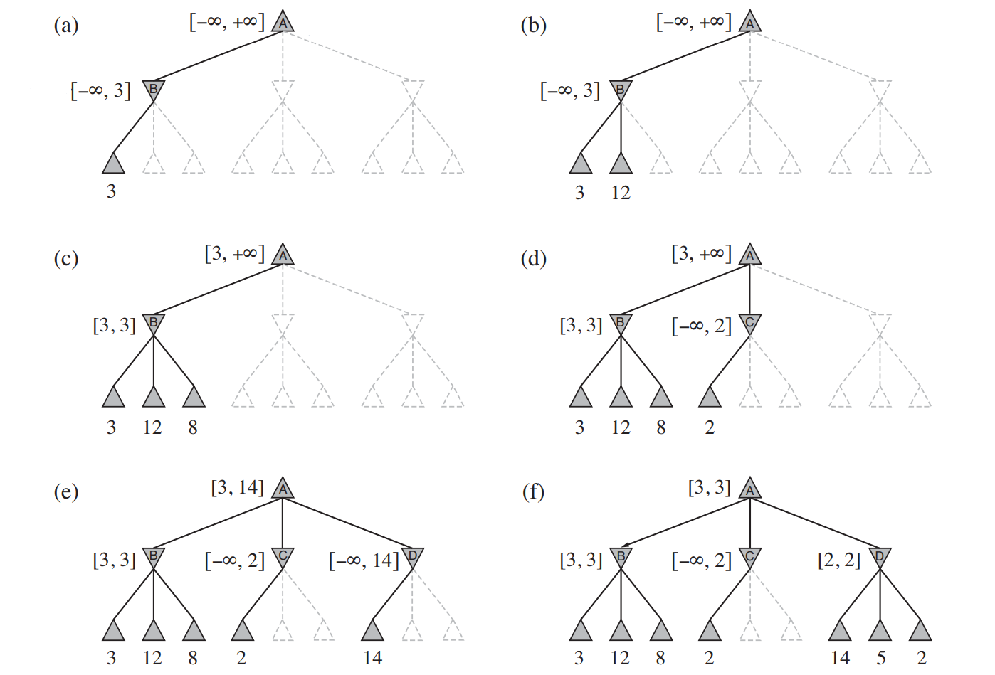
The idea of alpha-beta pruning comes from a very simple observation - in some cases, we don’t need to find all successors’ utilities to calculate the minimax value at a node. For instance, in the fig above, when we see the maximum minimax value at $C$ is 2, we know its minimax value must be smaller than $B$’s minimax value (which is 3) and we can ignore the other two nodes (dash line) under $C$.
If Player has a better choice than $n$, $n$ will never be reached in actual play. Therefore, once we find enough information about $n$ to reach this conclusion, we can prune it.
Below shows a general case for alpha-beta pruning:
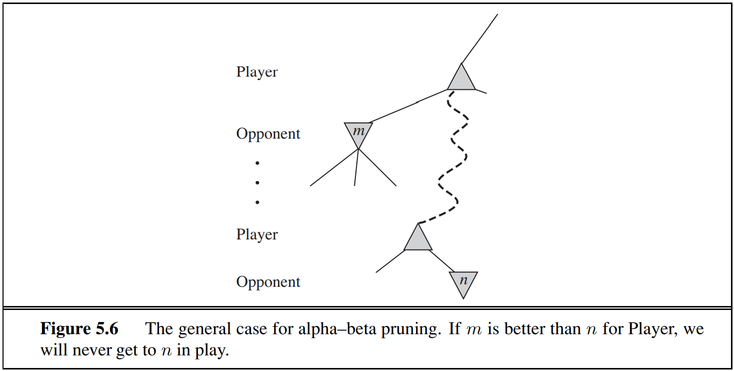
$\alpha=$ the minimax value of the best choice (max-value) we have found so far at any choice point along the path for MAX
$\beta=$ the minimax value of the best choice (min-value) we have found so far at any choice point along the path for MIN
Alpha-beta pruning update the $\alpha$ and $\beta$ as it goes along and prunes the remaining branches at a node as soon as the value of the current node is known to be worse than the current $\alpha$ or $\beta$ for MAX and MIN respectively.
def maxValue(s, alpha, beta) -> int:
    """
    returns an integer represent the minimax value at current state (or the last value before the node is pruned)
    """
    if TERMINAL_TEST(s): return UTILITY(s)
    minimaxVal = -1 * float("inf")
    for a in ACTION(s):
        minimaxVal = max(minimaxVal, minValue(RESULT(s, a), alpha, beta))
        if minimaxVal >= beta:      # Since the MIN agent is optimal, this scnerio will never occur
            return minimaxVal       # the following expansion is pruned
    return minimaxVal

def minValue(s, alpha, beta) -> int:
    """
    returns an integer represent the min minimax value at current state (or the last value before the node is pruned)
    """
    if TERMINAL_TEST(s): return UTILITY(s)
    minimaxVal = float("inf")
    for a in ACTION(s):
        minimaxVal = min(minimaxVal, maxValue(RESULT(s, a), alpha, beta))
        if minimaxVal <= alpha:     # Since the MAX agent is optimal, the MAX agent will never reach this node (as there exist better path)
            return minimaxValue     # the following expansion is pruned
    return minimaxValue
To start searching from the root, use maxValue(root, -1 * float("inf"), float("inf"))
5.4 Backtracking
Backtracking is a way to prune the search space. When we are searching through a search space, sometimes we can make sure the current solution is impossible when we haven’t reach the end of action sequence.
Suppose a game need 4 actions to make up an action sequence, we can sometimes know we will lose when playing only 2 actions yet. In this case, we can stop searching and go back to previous step and choose another action to play. (this is the reason why it is called Backtracking)
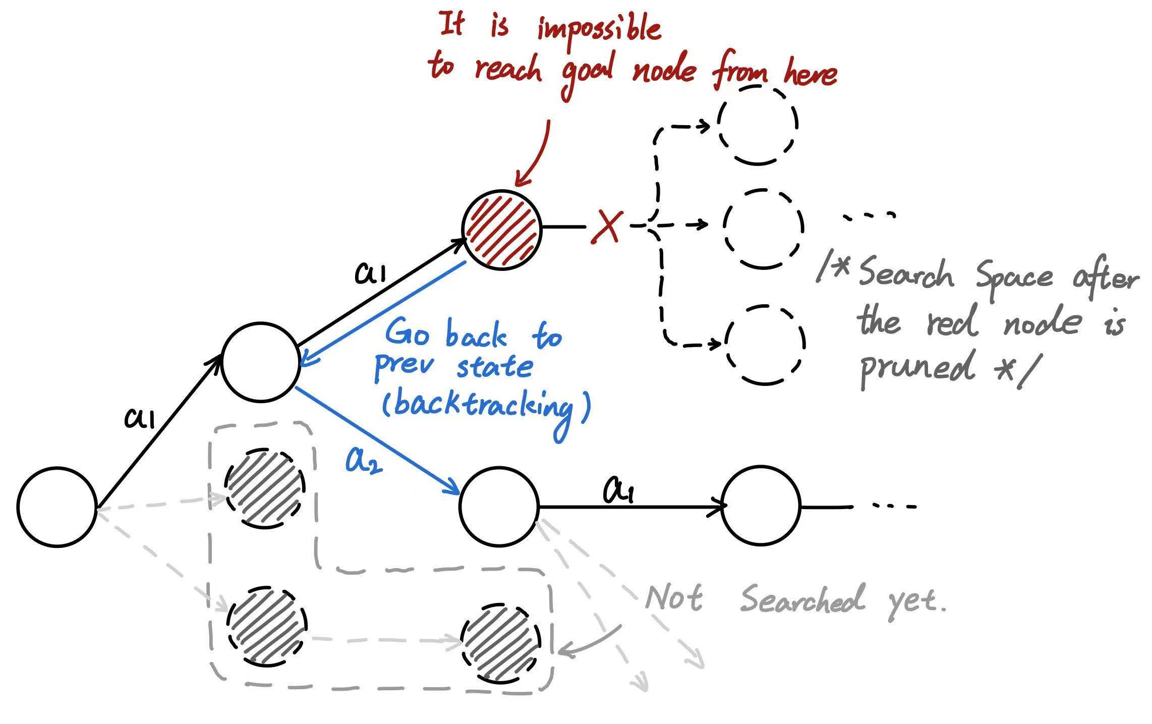
The effect of backtracking will be more significant if we can identify whether it is possible or not to get to goal node from a shallower node. In such situation, much of the search space will be pruned.
A famous problem that can be solved by Backtracking is the “eight queens” problem. Detailed description of a more general case (n-queen problem) is in this link: UVA-11195 Another n-Queen Problem.
def nQueen(state, currCol):
    if currCol == len(state): return 1

    resultState = 0
    for candidate in range(len(state)):
        if isValidState(state, candidate, currCol):
            newState = state[:]
            newState[currCol] = candidate
            resultState += nQueen(newState, currCol + 1)
    return resultState

def isValidState(state, candidate, currColumn):
    if candidate in state: return False     # are queens on the same row
    for i, position in enumerate(state):
        if i >= currColumn: break
        if abs(position - candidate) == (currColumn - i):
            return False                    # are queens on the same diagonal
    return True
