
报告错误
如果你发现该网页中存在错误/显示异常,可以从以下两种方式向我们报告错误,我们会尽快修复:
- 使用 CS Club 网站错误 为主题,附上错误截图或描述及网址后发送邮件到 286988023@qq.com
- 在我们的网站代码仓库中创建一个 issue 并在 issue 中描述问题 点击链接前往Github仓库

The Relationship between Searching and AI
As we have mentioned in chapter 1 and 2, an Intelligent Agent can maximize the utility in a given environment by control its behavior. Searching Algorithm is a very useful algorithm to find the sequence of actions that will maximize the utility.
Terminologies
| Term | Explanation |
|---|---|
| State | One status of environment, which can be represented using a series of parameters |
| State Space | All the states an environment can have. The state space can either be finite or infinite. |
| Action | The behavior of Agent. Usually Action can change the State (note: not always). |
| Fringe | The states in state space that is about to explore (expand) by the searching algorithm. |
| State Transition Function | The function that describe how state change between each other (how state transit). |
| Successor | The states that directly resulted from current state. $\text{currState}\quad \underrightarrow{Action} \quad \text{Successors}$ |
3.0 How do We Evaluate a Search Algorithm
We can evaluate a searching method in several aspects, as shown below:
- Consistency, given a State Space with Goal State in it, the algorithm MUST be able to find an action sequence that leads to the goal state.
- Optimality, Given a State Space that has Goal State in it, the searching algorithm MUST be able to find the Best Action Sequence that can lead to the Goal State
- Time Complexity, how many computation time it takes for the algorithm to find the Best Action Sequence to the Goal State
- Space Complexity, how many memory it use for the algorithm to find the Best Action Sequence to the Goal State.
3.1 Breadth First Search (BFS)
BFS is both Consistent and Optimal.
In the BFS algorithm, The shallowest state in state space is expanded first.
Due to this feature, when there are multiple goal states in the state space, the BFS can always find the shallowest goal state. Therefore, when all the actions have same cost, the BFS can always find the action sequence to goal state that have least cost.
The fringe of BFS is a Stack where FIFO policy applies.
Code Example
def breadthFirstSearch(initialState, getSuccessor, getValidActions):
    """
    :param initialState: The Initial State of problem (sometimes the 'current state')
    :param getSuccessor: The State Transition Function that return the successors given the current state and action
    :param getValidActions: A function that takes current state and return a list of valid actions under current state
    """
    fringe = stack()
    exploredStates = set()

    # Add the Initial State into the Fringe before Searching Actually Start.
    fringe.push(initialState)
    while len(fringe) > 0:
		currState = fringe.pop()
        if currState in exploredStates: continue
        else: exploredState.add(currState)

        # Do Something Here

        for action in getValidActions(currState):
            # Add Successor States into the fringe
            successor = getSuccessor(currState, action)
            if successor not in exploredStates: fringe.push(successor)
| Pros | Cons |
|---|---|
| The Optimality of Searching Result - the nearest goal state will always return first | High Space Complexity - The BFS algorithm requires much memory to maintain the fringe. Suppose each state leads to $3$ successors, when searching on a tree with height $10$, the fringe will have a size of $3^{10}\approx 60000$. (Space Complexity $O(m^n)$) |
| Easy to implement - no complex data structure required, the foundation of most searching algorithms | High Time Complexity - Suppose the goal state is at depth $n$, and on average each state has $m$ successors, the time complexity of BFS will be $O(m^{n+1})$ |
3.2 Depth First Search (DFS)
The DFS algorithm will First expand the Deepest node in the State space
Depth First Search Algorithm need Much Less Space to search all the nodes in a specific depth comparing to BFS, but it is not a great searching algorithm since it is not Optimal. In other words, the DFS will not return the optimal solution first.
In the DFS, the Fringe is a Queue, which applies the FIFO policy.
def depthFirstSearch(initialState, getSuccessor, getValidActions):
    """
    :param initialState: The Initial State of problem (sometimes the 'current state')
    :param getSuccessor: The State Transition Function that return the successors given the current state and action
    :param getValidActions: A function that takes current state and return a list of valid actions under current state
    """
    fringe = queue()    # The only difference between BFS and DFS
    exploredStates = set()

    # Add the Initial State into the Fringe before Searching Actually Start.
    fringe.push(initialState)
    while len(fringe) > 0:
		currState = fringe.pop()
        if currState in exploredStates: continue
        else: exploredState.add(currState)

        # Do Something Here

        for action in getValidActions(currState):
            # Add Successor States into the fringe
            successor = getSuccessor(currState, action)
            if successor not in exploredStates: fringe.push(successor)
3.2.1 Deep Limited Search
3.3 UCS Uniform Cost Search
There is a common problem in BFS and DFS: They don’t care the ACTUAL COST of action sequence to the goal state. Though BFS will return the Shortest action sequence to goal state, the shortest action sequence may not be the action sequence with lowest cost, like the example below shows:
The number inside each grid is the cost to go through that grid, $S$ is the initial state and $G$ is the goal state. In this case, the shortest action sequence $A$ has a Much Higher cost comparing to the min-cost action sequence $A^*$.
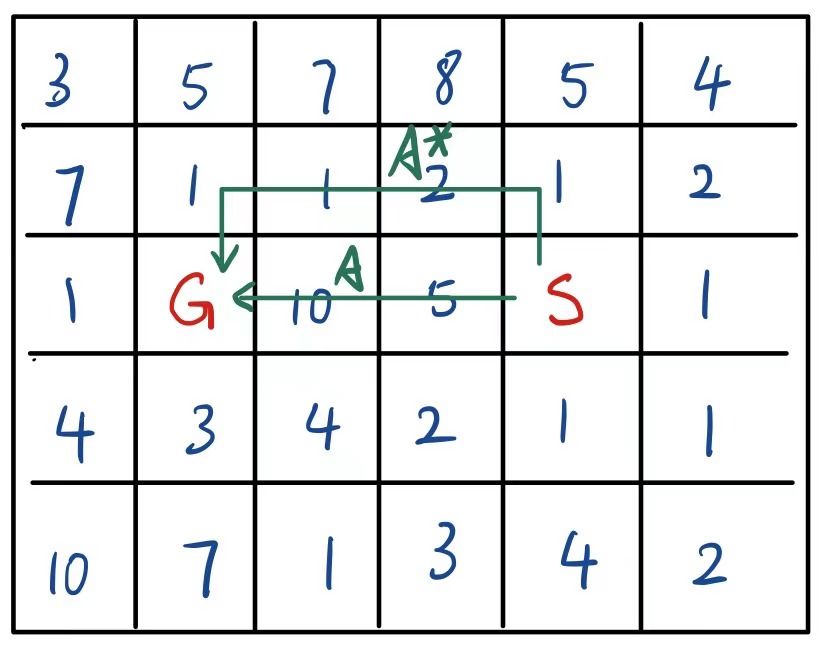
To solve this problem, we use the UCS to search through the state space, which will ALWAYS explore the state with minimal cumulative cost. To implement this feature, the fringe of UCS is a priority queue, where the cumulative cost is the weight to sort priority queue.
This stratagy is somehow similar to the stratagy used by Min Span Tree.
def uniformCostSearch(initialState, getSuccessor, getValidActions, getActionCost):
    """
    :param initialState: The Initial State of problem (sometimes the 'current state')
    :param getSuccessor: The State Transition Function that return the successors given the current state and action
    :param getValidActions: A function that takes current state and return a list of valid actions under current state
    :param getActionCost: A function that will return cost of action given action and current state
    """
    fringe = []    # The only difference between BFS and DFS
    exploredStates = set()

    # Add the Initial State into the Fringe before Searching Actually Start.
    # Instead of storing state directly in the fringe, we will use a tuple to store state, where the
    # 0th param of tuple is cumulative cost
    # 1th param of tuple is the state

    heapq.heappush(fringe, (0, initialState))	# The initial cost is 0
    while len(fringe) > 0:
		cost, currState = heapq.heappop(fringe)
        if currState in exploredStates: continue
        else: exploredState.add(currState)

        # Do Something Here

        for action in getValidActions(currState):
            # Add Successor States into the fringe
            successor = getSuccessor(currState, action)
            if successor not in exploredStates:
                deltaCost = getActionCost(currrState, action)
                heapq.heappush((cost + deltaCost, successor))
In Python, the priority queue is implemented by internal library heapq.
Tree Search v. Graph Search
Tree Search and Graph Search are two types of searching algorithms. Tree search is like a tree in graph theory - ther is no loop insied the state transition space. Therefore, any explored state node will NEVER be explored again.
Graph Search, on the other hand, does not record the explored nodes in the state space. Everytime a Graph Search algorithm expand a node, all of its successor states will be added into the fringe. The cycle inside the graph is redundant part of a graph, which exists whever there is more than one way to get from one state to another.
Symbols Used below
Symbol Meaning $f(n)$ The evaluation function for node $n$ $g(n)$ The total cost to get to $n$ from initial state (node) $h(n)$ The heuristic function that estimate the total cost to get to goal state from $n$ $c(n, a, n’)$ The actual cost of getting from $n$ to $n’$ through action $a$
3.4 Informed Search
Greedy search is a form of informed search, that is, information other than the definition of search problem is used to find the goal state. The informed search can find solutions more efficiently than an uninformed strategy.
Among many types of informed search, the greedy search is one of the most general approach.
Each node is evaluated using an evaluation function $f(n)$. The evaluation function $f(n)$’s value is considered as a cost estimate. In Greedy Search, the node in fringe with lowest evaluation will be expanded first. For most of the evaluation function, there is a part of heuristic function (denoted as $h(n)$) that helps to estimate the cost from current node to the goal state.
\[h(x) = \text{The estimated cost of the cheapest path from state node } n \text{ to the Goal State}\]A heuristic function is non-negative, problem specific function and there is only one constraint: if $n$ is a goal state, then $h(n) = 0$.
3.4.1 Greedy Best-first Search
Greedy Search evaluate the nodes only using the heuristic function $h(x)$. That is, the evaluation function $f(n)$ is equal to the heuristic function $h(x)$.
A simple greedy best-first search’s tree search version is incomplete even in a finite state space. It’s graph search version is complete in finite state space.
If the branching factor of graph is $\alpha$, then Greedy Search’s tree version’s worst time complexity will be $O(\alpha^m)$, where $m$ is the maximum depth of the search space. However, the actual time complexity of Greedy Best First Search will rely on the quality of heuristic function.
3.5 A* Search
A* Search evaluates nodes in search space by combining $g(n)$, the cost to reach the node, and $h(n)$, the estimated cost to get from the node to the goal. In A* search, the evaluation function $f(n)$ can be written in this form:
\[f(n) = g(n) + h(n)\]In this case, $f(n)$ is the estimated cost of the cheapest solution through $n$.
Provided that the heuristic function $h(n)$ satisfies certain conditions, A* search is both complete and optimal.
The A* search algorithm is identical to Uniform-Cost-Search except that A* uses $g(n) + h(n)$ while UCS use $g(n)$.
3.5.1 Conditions for optimality: Admissibility and Consistency
Admissibility
The evaluation function of A* search is $f(n) = h(n) + g(n)$, the admissibility means that for any node $n$, the evaluation function $f(n)$ Never Overestimate the actual cost of a solution along the current path through $n$.
Consistency
The heuristic function $h(n)$ is consistent if for every node $n$ and every successor $n’$ of $n$ generated by any action $a$, the estimated cost of reaching the goal from $n$ is no greater than the step cost of getting to $n’$ plus the estimated cost of reaching the goal from $n’$.
\[h(n) \leq c(n, a, n') + h(n')\]*3.6 Prove the Optimality of A* Search
- Tree search version of A* search is optimal if $h(n)$ is admissible.
- Graph search version of A* search is optimal if $h(n)$ is consistent.
Below will show the proof of second arguement.
Lemma 0: If $h(n)$ is consistent, then the values of $f(n)$ along any path are nondecreasing.
Suppose $n’$ is a successor of $n$, then $g(n’) = g(n) + c(n, a, n’)$ for some action $a$. Therefore, we have
\[f(n') = g(n') + h(n') = g(n) + c(n, a, n') + h(n') \geq g(n) + h(n) = f(n)\]Lemma 1 Whenever A* selects a node $n$ for expansion, the optimal path to that node has been found.
Suppose this is not the case and there exist a path passing through node $n’$ and reach $n$ with lower cost, there will exist a conflict: Accroading to lemma 0, the $f(n)$ along any path are nondecreasing, then $f(n’) \leq f(n)$, which means that $n’$ is explored before $n$ is selected by A* algorithm.
From these two lemma, we can draw conclusion that A* search expand nodes in the non-decreasing order of $f(n)$. For goal node, $f(n) = g(n)$ (as $h(n) = 0$), so the first selected goal node must be the goal node with minimum $g(n)$.
